1. Introduction
This document is intended to provide the LAT
collaborators with sufficient information to perform data analysis during LAT
integration. It is intended for users who are familiar with the LAT instrument,
however a brief overview is provided.
Most of the information in this document is
either copied from the website of Instrument Analysis Workshop presentations,
or existing LATDocs documents. A list of references is provided in Resources, section 12.
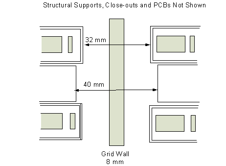
The Large Array Telescope (LAT) is an
integrated instrument consisting of 16 towers set into a 4x4 grid. Each tower consists
of a Tracker (TKR), Calorimeter (CAL), and Tower Electronics Module (TEM). The
LAT is shown in Figure
1. The 16 towers are surrounded by an
Anti-Coincidence Detector (ACD) which is surrounded by a micro-meteorite shield.
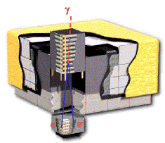
Figure 1: The LAT
The following paragraphs provide a brief
description of how the major components are used during pre-launch tests and
are shown in Figure
2.
The ACD is mostly used to either identify charged
particles for cosmic ray calibration runs, or to reject charged particles
during Van de Graaff photon calibration runs.
The TKR’s function is to
reconstruct the original direction of travel of either incoming photons (from 18
MeV photons from a Van de Graaff generator) or of charged particles (cosmic
rays).
The CAL’s function is to measure
the energy deposited by incoming charged particles, either from photon pair
creation or cosmic rays.
The TEM assembles trigger primitives from the TKR and CAL (or simulated input)
to determine whether or not there has been an event in the LAT. If so, it
alerts the GLAST Electronics Module (GEM). It also communicates with the Event
Builder Module. Trigger parameters are stored in the TEM.
The GEM (also referred to as the GLAST LAT Trigger -
GLT) responds to a TEM’s message that an event has been detected and decides
whether or not to generate a trigger. The GEM is an important component when
performing Dead Time and Trigger analyses.
The Anti-Coincidence Detector Electronics
Module (AEM) performs the same
function for the ACD as the TEM does for the TKR and CAL detectors.
The Event Builder Module (EBM) communicates with the
GEM, TEM and AEM.
The
Global-trigger/ACD-module/Signal-distribution Unit (GASU) performs the highest logic
level of event decision making, and comprises the AEM, GEM and EBM.
The Power Distribution Unit (PDU) supplies DC current to
operate the electronics.
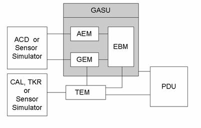
Figure 2: Principal LAT Components (Block Diagram)
NOTE: Real detectors (ACD, TKR,
CAL) can be replaced by simulated
input that mimics the behavior of the physical detectors beginning at the
cables that readout the detectors. Although the Front End Electronics (FEE) are
not simulated, a pattern can be created to generate events.
Data taking with cosmic ray muons will occur with 1, 2, 4,
6, 8, 10, 12, 14 and 16 Flight Modules (FMs) installed in the LAT grid. The
first position filled is position #0. The second position filled is #4. 15
hours of cosmic ray data taking (plus one hour with zero suppression OFF) occurs
every time towers are added to the LAT. 16 hours of data taking with Van de
Graaff photons occurs for tower A. Please refer to LAT-MD-00575 for detailed
information on data taking during integration. Figure 3 shows the tower positions filled in each
data taking configuration. Note that shaded squares indicate a tower
installed in the grid.
For each hardware configuration there will be
a baseline cosmic ray data-taking run for which the hardware is configured with
nominal settings (please refer to the Nominal Register Settings in section 5) for ground analysis for the integrated hardware
(towers).
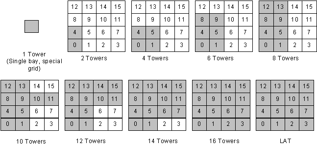
Figure 3:
Tower Placement for Cosmic Ray Data Taking
Monte Carlo
simulations for Flight Modules will be performed for 1, 2, and 8 towers, and the
fully integrated LAT grid, as shown in Figure 4.
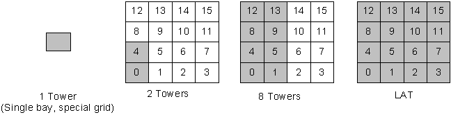
Figure 4: Grid
Tower Positions for Monte Carlo Simulations
The global instrument coordinate system for
the LAT is consistent with the coordinate system for the observatory. It is a
right-handed coordinate system with the Y-axis parallel to the
solar panel axis, the Z axis normal to the
planes of the TKR, CAL,
and Grid (i.e., parallel to the “bore sight”), and the X axis is mutually
perpendicular to Y and Z. The positive Z-axis points from the CAL to the TKR. Particles entering the
instrument at normal incidence are thus oriented along the -Z direction (please
see Figure
5).
The point X=Y=0 is at the center of the Grid.
The Z=0 plane is at the top face of the Grid, between the TKR and CAL units on the TKR side of the Grid. The
TKR silicon plane closest
to Z = 0 is at Z = +33 mm; the crystal plane closest to Z = 0 is at Z = -46 mm.

Figure 5: LAT
Tower Numbering and Grid
Coordinate System
2.1.
ACD Geometry and Numbering Scheme
The active elements of the ACD consist of 89
tiles and 9 ribbons. (A figure will be added later.)
The tracker is made up of 19 trays
comprising 36 planes as shown in Figure 6. The 36 planes are mated into 18 layers.
The TKR trays are numbered in increasing
order with increasing Z. Each tray has two active planes, except the top half
of the top tray (+Z) and bottom half of the bottom tray.
A tray measures in either the X or Y direction, i.e.,
has an X or Y view. To get X and Y
information, planes from two adjacent trays are electronically combined. Mated X
and Y planes are about 2 mm apart. This arrangement leaves the top-most and
bottom-most planes without a partner and without silicon detectors.
A tray with detector strips
physically parallel to the Y axis is an X tray: it measures the X coordinate (has
an X view) and is called an X tray. Most planes have an embedded tungsten foil for
g conversion: The top 12 X and Y
pairs have a thin foil (3% of X0),
the next four have a thick foil (18% of X0),
and the bottom two X and Y pairs have no tungsten.
The active region of each TKR plane is
comprised of 16 square Silicon Strip Detectors (SSDs - please see Figure 7). Each SSD has 384 conducting strips. Four
SSDs are end-joined to make a ladder with the four SSDs in a given ladder joined
mechanically and electrically to make 384 long strips. Four ladders per plane
laid side-by-side make up a total of 1536 strips per plane. Each plane is about
360 mm by 360 mm in area.
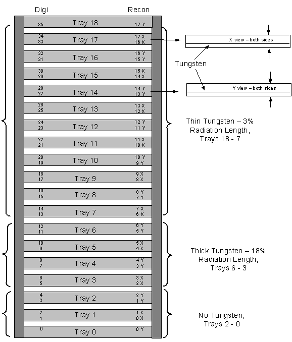
Figure 6: TKR Tower Numbering Scheme.
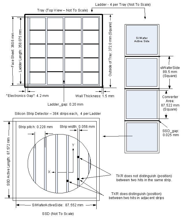
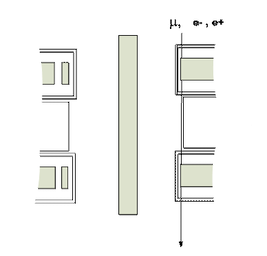
Figure 7: TKR Plane Physical Details (X-View)
Each CAL module is made up of 96 crystals
oriented in a hodoscopic configuration of 8 layers of 12 crystals each. In
contrast to a TKR plane, a CAL crystal makes its coordinate measurement along
its principal axis: an X crystal has its principal axis along the X direction,
as shown in Figure 8.
Each crystal has two PIN diodes at each end
for reading out the signal. Each PIN diode (at either end) reads out for either
the low or high energy measurement. The low energy PIN has an area four times
greater than the high energy PIN.
The CAL layers are numbered from 0 – 7 in
increasing order with decreasing Z. The CAL layers closest to the TKR is plane
0. CAL layers 0 has X crystals; CAL layers 7 has Y crystals. Each CAL crystal
is read from each end, and each crystal end is either plus or minus: the end
with the larger value of the coordinate is the “plus” end and the end with the smaller
value of the coordinate is the “minus.”
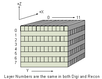
Figure 8: CAL Crystal Layer Numbering and Orientation
Figure
10 shows an accurate representation of a CAL
module.
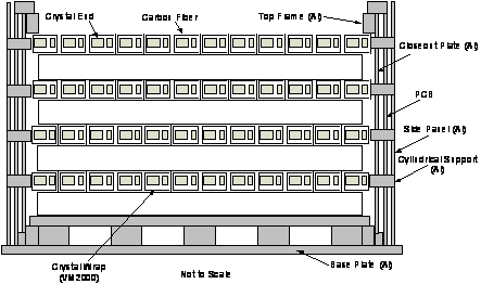
Figure 9: CAL Module Cross
Section
Figure 10 shows a close-up view of the displacement of CAL
crystal ends of two adjacent CAL modules. It is important to note that crystal
ends that face each other are at a different spacing than the closest crystals
in adjacent modules that are parallel to each other.
Figure
10: Zoom of Region
between Two Adjacent CAL Modules (3 layers shown)
The CAL
crystal profile is shown in Figure 11 along with the dimensions of a CAL
crystal, including its carbon fiber enclosure.
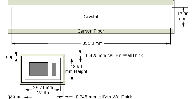
Figure
11: CAL
Crystal Dimensions
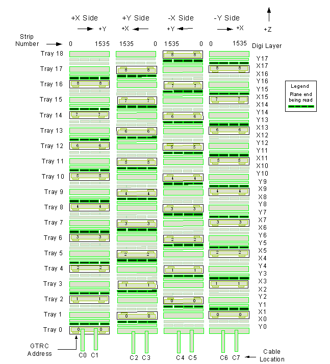
Table 1 lists the number of readout channels
(active elements) for the ACD, TKR and CAL in a 1, 2, 4, 8, and the full LAT
configuration. Note that the ACD front-end PCBs actually have 216 channels, but
because each tile is read by 2 PMTs that are assembled with a logical OR, the
number of tiles that can be read out is actually 108. With a total number of 97 tiles and ribbons, some channels are not
used.
Table 1: Detector Readout Channels
|
|
|
|
|
|
|
|
|
|
|
|
1 Tower
|
|
|
36 / 55,296
|
96 / 384
|
|
2 Tower
|
|
|
72 / 110,592
|
192 / 768
|
|
4 Tower
|
|
|
144 / 221,184
|
384 / 1536
|
|
8 Tower
|
|
|
288 / 442,368
|
768 / 3072
|
|
LAT
|
89/178
|
8/16
|
576 / 884,736
|
1536 / 6144
|
To be written.
3.2.
TKR Readout Sequence
Data from each silicon plane is read out by
24 GTFE ASICs located in a Multi-Chip-Module (MCM), controlled by 2 GLAST
Tracker Readout Controllers (GTRC). There are 2 (GTRC 0 and GTRC 1) per plane
or 4 per tray, except trays 0 and 18 (please see Figure 19). The two GTRCs are situated at the edge
of the plane. GTRC 0 (RC0) is defined as being closest to where strip 0 is
located. RC1 is defined as where strip 1535 is located. The default mode is to
read from both ends. The readouts of a TKR are carried through eight cables
(please see Figure
12).
If any shaper-out signal of a channel in a
GTFE chip is over threshold, a trigger request (TREQ) signal is issued and
transferred to the TEM, which then checks the trigger status. If a trigger
condition (3-in-a-row) is satisfied, the TEM sends the trigger request acknowledge
(TACK) signal to all planes to latch hit strip data into GTFE event buffers. Each
GTFE has 4 event buffers. Note that it
is not the TREQ but the TACK signal that starts the Time over Threshold (ToT)
counter in the GTRC.
The TEM sends the READ-OUT command and
transfers event data from GTFE event buffers to GTRC event buffers. A GTRC
event buffer is limited to 64 hit-strips. The GTRC has 2 buffers. The TEM sends
the TOKEN signal and transfers event data from the GTRC event buffers to the
TEM one plane at a time. The GTRC waits to send data until the process of the READ-OUT
command finishes, and the ToT counter terminates. The ToT counter saturates at
1000 clock cycles (= 50 μs). In a case where the ToT counter overflows, the
GTRC will start to send data at the overflow point (1000 clock cycles).
The TKR mapping scheme is shown in Table
2. This table maps the TKR physical
information in LDF, digi and recon files. Note that GTRC value is an address. These
numbers are unique taken in combination with the cable controller. Figure 12 shows the four faces of the TKR. A typical user
does not need to know the information in electronics space. This table is intended to serve as a
reference for hardware-oriented people. Before using the Electronics Space
information, always verify that it is the latest information in the TEM manual.
Table 2: TKR Mapping between Physical and Electronics Space. Note
that “X” or “Y” Means Measured Coordinate, T= Top Side of Tray, B=Bottom Side
of Tray
|
|
|
|
|
|
|
|
|
|
|
|
|
|
18/B
|
35
|
17
|
Y
|
4,5
|
8
|
|
17/T
|
34
|
17
|
X
|
6,7
|
8
|
|
17/B
|
33
|
16
|
X
|
2,3
|
8
|
|
16/T
|
32
|
16
|
Y
|
0,1
|
8
|
|
16/B
|
31
|
15
|
Y
|
4,5
|
7
|
|
15/T
|
30
|
15
|
X
|
6,7
|
7
|
|
15/B
|
29
|
14
|
X
|
2,3
|
7
|
|
14/T
|
28
|
14
|
Y
|
0,1
|
7
|
|
14/B
|
27
|
13
|
Y
|
4,5
|
6
|
|
13/T
|
26
|
13
|
X
|
6,7
|
6
|
|
13/B
|
25
|
12
|
X
|
2,3
|
6
|
|
12/T
|
24
|
12
|
Y
|
0,1
|
6
|
|
12/B
|
23
|
11
|
Y
|
4,5
|
5
|
|
11/T
|
22
|
11
|
X
|
6,7
|
5
|
|
11/B
|
21
|
10
|
X
|
2,3
|
5
|
|
10/T
|
20
|
10
|
Y
|
0,1
|
5
|
|
10/B
|
19
|
9
|
Y
|
4,5
|
4
|
|
9/T
|
18
|
9
|
X
|
6,7
|
4
|
|
9/B
|
17
|
8
|
X
|
2,3
|
4
|
|
8/T
|
16
|
8
|
Y
|
0,1
|
4
|
|
8/B
|
15
|
7
|
Y
|
4,5
|
3
|
|
7/T
|
14
|
7
|
X
|
6,7
|
3
|
|
7/B
|
13
|
6
|
X
|
2,3
|
3
|
|
6/T
|
12
|
6
|
Y
|
0,1
|
3
|
|
6/B
|
11
|
5
|
Y
|
4,5
|
2
|
|
5/T
|
10
|
5
|
X
|
6,7
|
2
|
|
5/B
|
9
|
4
|
X
|
2,3
|
2
|
|
4/T
|
8
|
4
|
Y
|
0,1
|
2
|
|
4/B
|
7
|
3
|
Y
|
4,5
|
1
|
|
3/T
|
6
|
3
|
X
|
6,7
|
1
|
|
3/B
|
5
|
2
|
X
|
2,3
|
1
|
|
2/T
|
4
|
2
|
Y
|
0,1
|
1
|
|
2/B
|
3
|
1
|
Y
|
4,5
|
0
|
|
1/T
|
2
|
1
|
X
|
6,7
|
0
|
|
1/B
|
1
|
0
|
X
|
2,3
|
0
|
|
0/T
|
0
|
0
|
Y
|
0,1
|
0
|
Figure
12: The Four Sides of the TKR Tower with Cables.
“X” or “Y” Means Measured Coordinate.
3.3.
CAL Readout Sequence
The CAL crystals are normally read from both
ends through a total of four cables – each crystal is read out by two cables,
one + and one -. Each crystal end has two PIN diodes, one large and one small,
for low and high energy, respectively. Each crystal end (left and right, or +
and -) has its own FEE pre-amplifier electronics assembly for a total of 192. Both
low and high energy signals go through a pre amp and shaper then a Track and
Hold gain multiplier and into an analog multiplexer and finally to the Analog
to Digital Converter (ADC). Each row of crystals has a GCRC for each end for a
total of 16. (There are 8 rows and each row is read out at both ends.) The 16
GCRCs feed four cables (and four GCCCs). The cables carry +X, -X, +Y and -Y
signals to the GCCCs. The two X GCCCs
combine +X and -X information to produce X0, X1, X2, X3 signals; the Y GCCCs do
the same to produce Y0, Y1, Y2, and Y3. A simplified FEE schematic
diagram is shown in Figure
13. The calibration charge injection
signal is fed to the front end of these pre amps.
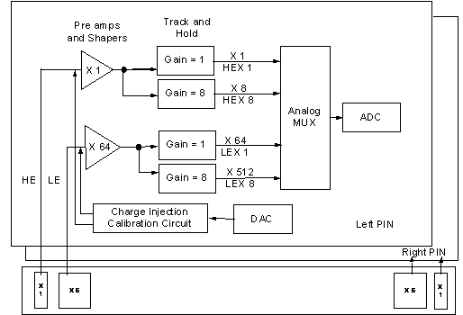
Figure 13: CAL FEE Simplified Schematic Diagram
Table
3 shows the gain stages.
Table 3: CAL FEE Signal Gain Characteristics
|
|
|
|
|
|
|
|
Low Energy
|
X 6
|
X 64
|
X 1
|
LEX1
|
64
|
|
X 8
|
LEX8
|
512
|
|
High Energy
|
X 1
|
X 1
|
X 1
|
HEX1
|
1
|
|
X 8
|
HEX8
|
8
|
Figure 14 shows how the energy ranges overlap. During
cosmic ray data taking on the ground most of the events fall within the low
range diodes.

Figure 14: CAL Channel Signal Range Energy Overlap
Table 4 maps the locations of layers and
crystal ends between the electronics space and the physical space. A typical
user does not need to know the information in electronics space. This table is intended to serve as a
reference for hardware-oriented people. Before using the Electronics Space
information, always verify that it is the latest information in the TEM manual.
Table 4: CAL Mapping between Physical and Electronics Space
|
|
|
|
|
|
|
|
|
|
|
|
|
|
|
0 / X
|
0
|
0
|
0,2
|
0
|
|
1 / Y
|
1
|
1
|
1,3
|
0
|
|
2 / X
|
2
|
2
|
0,2
|
1
|
|
3 / Y
|
3
|
3
|
1,3
|
1
|
|
4 / X
|
4
|
4
|
0,2
|
2
|
|
5 / Y
|
5
|
5
|
1,3
|
2
|
|
6 / X
|
6
|
6
|
0,2
|
3
|
|
7 / Y
|
7
|
7
|
1,3
|
3
|
The CAL readout cables and the associated GCCC are
shown in Figure
15.
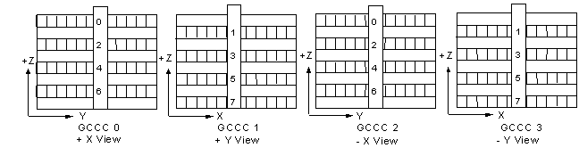
Figure 15: The Four Sides of the CAL Module with
Cables
The Trigger inputs from the ACD, CAL and TKR
are processed by the GEM. The GEM decides whether to read out an event, or not,
based on all inputs received. Therefore trigger primitives can be issued but
may lead to no data latched if the GEM decides that all necessary conditions
have not been met.
Any of the three detectors (ACD, CAL and
TKR) can issue a trigger request (TREQ) but data is only latched from the
detector buffers if the GEM logic is satisfied that a trigger acknowledge
(TACK) is warranted.
The ACD signals are usually used as a veto
for charged particles. However, the CNO signal can be used to trigger on heavy
nuclei (mostly used for calibrations). During ground testing we can only test
the CNO signal through charge injection. Another useful concept one has to keep
in mind is that Regions Of Interest (ROI) can be defined using the ACD tiles.
So a number of tiles can be logically grouped for trigger/veto purposes.
The TKR trigger logic requires at least one
hit above a predetermined threshold in three consecutive XY planes (six planes).
The CAL trigger logic requires at least one
hit above a predetermined threshold in any of the crystals. One can have a low energy trigger and a high
energy trigger. For ground testing with cosmic rays the nominal CAL low-energy
trigger is already too high and one must lower the discriminator thresholds or
use the TKR trigger, instead.
During ground testing there will be a
pattern generator (software) that will produce several trigger rates from a few
Hz to tens of kHz. These solicited triggers will be overlaid with the
nominal trigger conditions (e.g. TKR trigger) to study the behavior of the
trigger and data flow system.
To trigger on a set of trigger inputs coming
from different detectors, they must all fall within the same time coincidence
window, but the system must not be busy (already reading an event). Note that
during ground testing, in order to cope with rates greater than 1.5 kHz, one
may have to prescale (discard) events. Note that an otherwise “triggerable”
event may not be latched because it was prescaled away, or because the
instrument was busy. Trigger information the GEM reports:
·
Number of triggered events not passing the
prescalers (Prescale count – 24 bits)
·
Number of triggered events passing the
prescalers, but lost due to the LAT being busy (Discarded counts – 24 bits)
·
Number of triggered events read out (Sent count
– 16 bits)
For the TKR, the hit threshold is also the
trigger threshold. The threshold is that six consecutive planes must be fired.
Nominal trigger rate on the ground (no ACD) is roughly 25 Hz (TBR) for each TKR
tower for cosmic ray analysis.
Trigger studies are performed as illustrated
in Figure 16. Actual tracker trigger primitives are received by
the TEM, which makes a trigger request, and then by the GEM, which evaluates
the request and either does, or doesn’t, issue a trigger acknowledge. Trigger
request information does not include which strip was fired (and initiated the
trigger request). Therefore, it is useful to compare real trigger requests with
simulated trigger requests.
When a tracker requests a trigger, the
possibility exists that the charge will not be held when the data is latched.
This should be investigated during timing studies.
Without Flight Software (FSW) there are
possible timing problems, such as difficulty in relating GEM time counters to
the Online 60Hz and 20 MHz event time stamps. The 20 MHz time stamp is applied
when the event is moved from the Event Builder, and this time may increase as
events queue up. Above 300 Hz the GEM Delta event time is usable. It is the
time between event (n-1) and event n. It is a 16-bit counter that saturates at
3.2 ms.

Figure 16: Trigger Studies of Real Triggers vs. MC
Simulations
All three subsystems have preamps that put
out shaped pulses that peak at different times after the entrance time (t0) for the particle into the LAT.
Any one of the three detectors can cause the
GEM to issue a TACK which latches the buffered data of all three detectors
regardless of whether or not they issued a trigger request. The purpose of the
time delays is to ensure that the trigger window is open at the correct time to
receive data from all the detectors at the peak of the input pulses for a given
detector. Table
5 shows the different delays for the ACD,
CAL and TKR. The table is for the entire ACD but just one of the 16 tower
modules.
Table 5: Number of Timing Delay Registers
|
|
|
|
|
ACD
|
12 TREQ Delays
|
12 TACK Delays
|
|
CAL High
|
4 TREQ Cable Delays
|
1 TREQ Delay (OR of 4 inputs)
|
1 TACK Delay (applied to all 4 cables)
|
4 TACK Cable Delays
|
|
CAL Low
|
1 TREQ Delay (OR of 4 inputs)
|
|
TKR
|
8 TREQ Cable Delays
|
1 TREQ Delay (OR of 8 inputs)
|
1 TACK Delay (applied to all 8 cables)
|
8 TACK Cable Delays
|
Figure 17 shows the various time delay registers
that are available at the input to the GEM. CAL low and CAL high come in on the
same four cables, each with a cable delay. The two CAL high signals are
OR’d as are the two CAL low signals with
each line having a TREQ delay as input to the GEM. The TKR signals come in on
eight cables, each with a delay register. The eight signals are OR’d into one
line which has a delay register before input into the GEM. The ACD signals come
in through 12 lines, each with a delay in the GEM input.
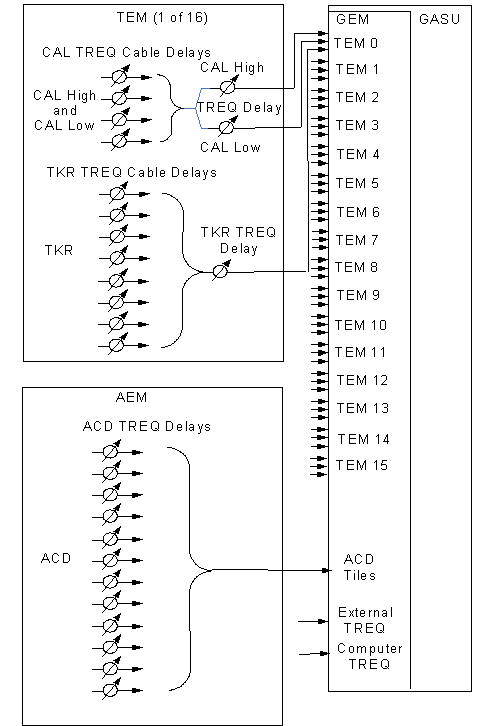
Figure 17: Conceptual Trigger Delay Adjustments
Diagram (GEM Inputs)
The GASU output (please see Figure 18) has an adjustable Trigger Window Width
register that feeds all three detectors with a single signal line. For the CAL
it passes through a TACK delay register before being split into four lines,
each with a CAL TACK cable delay. Likewise, the GASU output signal passes
through a TKR TACK delay before being split into eight lines, each with a TKR
TACK cable delay. For the ACD the GASU output signal splits into 12 lines, each
with an ACD TACK delay register.
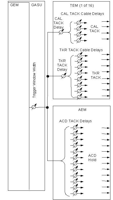
Figure 18: Conceptual Trigger Delay Adjustments
Diagram (GEM Outputs)
Dead time will be monitored with the Online
System and calculated with Offline tests. The dead time is always measured on
an event-by-event basis for the entire detector. If information is needed for dead time for individual systems, e.g.,
CAL/TKR/ACD, we will need to produce a special data taking run with only one
detector enabled.
When zero suppression is turned OFF, dead
time increases considerably. For example, the CAL, which dominates the dead
time, is expected to be at around 26 ms for flight
configuration and about 600 ms with zero
suppression OFF.
Live Time is 1/ Dead Time.
Every time a cosmic ray or gamma ray
interacts in the LAT, i.e., causes the LAT to trigger, further data taking is
disabled until the data from the event are read out. During the readout, the LAT is effectively
'dead' as a detector. The dead time per
event is small, probably about 20 microseconds, but the LAT will trigger
several thousand times per second on cosmic rays, so the fraction of the time
that the LAT is dead will be on the order of 10%. The rate of triggers on
cosmic rays will vary with orbital position. Also, during solar flares or even
possibly during extremely bright gamma-ray bursts, the dead time fraction could
become close to 1. The reason we care
about dead time is so that we can convert the rates of detections of gamma rays
from a given celestial sources into actual fluxes (numbers of photons per unit
area per unit time). In terms of optical
astronomy, this is roughly equivalent to the difference between seeing stars
and measuring their magnitudes. Keeping
track of live time is essential for getting the brightness correct.
There are hundreds of registers in the LAT.
Here we discuss only a few registers that one need be aware of for data
analysis.
5.1.
ACD Nominal Register Settings
To be written.
To be written.
To be written.
The ACD has 12 ACD TREQ delay registers
feeding into the GEM. There are also 12 ACD TACK delay registers applied to the
output of the GEM for ACD hold. Table 6 lists the nominal settings for the ACD
delays. Until test are performed assume that all 12 delays for the input or
output are equal.
Table 6: ACD Delay Register Nominal Settings
|
|
|
|
12 TREQ Delays
|
To be written
|
|
12 TACK Delays
|
To be written
|
To be written.
Nominal settings for the registers of
interest are described here. The
registers of interest are the GTFE registers MODE, DAC and MASK, and the GTRC
registers for GTFE_CNT, SIZE, and TOT_EN and time delays.
The GTFE threshold setting defines an energy
value above which the preamplifier in each channel integrates the charge
collected until the charge signal re-crosses the threshold as it drops. The
time the signal remains over the threshold is the ToT. Please see Figure 20.
Each strip hit in a silicon plane
contributes with a ToT value. A logical OR of all strips in the plane is used
to determine the value of the ToT per plane. ToT can be used to crudely
determine the amount of energy deposited on a TKR plane because its value is
dominated by the strip with the highest energy deposited. Channel-to-channel
variations exist and this is discussed further in the Calibrations Section, 6.2.
Each plane generates two ToT values because
it can be read out by 2 GTRC chips (please see Figure 19). The default configuration is to read 12
GTFEs with each GTRC: 12 GTFE chips read out by GTRC0 and 12 GTFE chips read
out by GTRC1. If a GTFE fails it can be by-passed and the split is modified
from the usual 12/12. Every data analysis run includes a report that states
what the GTRC split is, which is important for Timing and Trigger studies.
Figure 19: TKR FEE Readout Channel Splitting
The hit threshold can be set individually
for each GTFE with a default value of 0.25 of that of a Minimum Ionizing
Particle (MIP). The goal for the data taking with cosmic rays and VDG
accelerator is to have a uniform set of thresholds across all readout chips.
These are determined by measuring both the trigger capture efficiency and the
noise rate as a function of the discriminator DAC settings.
Figure 20: Shaper Output Time over Threshold
The GTFE and GTRC registers of interest are
shown in Table
7.
Table 7: TKR GTFE and GTRC Registers
|
|
|
|
|
|
GTFE
(Please refer to LAT-SS-00169 for further
details.)
|
Mode
|
2-bit
|
Left or Right mode (Is the GTFE read out
by the left or right GTRC)
|
|
Deaf mode ON / OFF (Is the GTFE deaf to
the GTFE beside it?)
|
|
DAC
|
7-bit +
7-bit
|
THR_DAC: (0-2 MIPS) Sets the threshold
level of the comparator. Range: about 0.05 -10 fC
|
|
CAL_DAC: (0-8 MIPS) Sets pulse height of
calibration strobe signal. Range: about 0.072-43 fC
|
|
Mask
|
64-bit
|
Channel mask
Trigger mask
Calibration mask
|
|
GTRC
(Please refer to LAT-SS-00170 for further
details.)
|
GTRC_CNT
|
|
Sets the number of GTFEs to read by
defining the LEFT/RIGHT split point. Range: 0-24. The default is 12 LEFT and
12 RIGHT. Please see Figure 19.
|
|
Size
|
|
Sets the maximum number of hits to get
from the GTFEs. Range: 0-64. The default is 64.
NOTE: Max hits/plane: 128 can be read using both LEFT and
RIGHT sides.
|
|
TOT_EN
|
1-bit
|
ENABLE TOT (1) or DISABLE TOT (0). The
default is 1.
|
Each TKR has a total of nine TREQ delays. Each TKR has a total of nine TACK delays. Table 8 lists the TKR delay register nominal
settings. Until test are performed assume that the cable delays for an input or
output are equal.
Table 8: TKR Delay Registers Nominal Settings
|
|
|
|
|
TREQ (8 – 1 per cable)
|
0
|
|
|
OR’d TREQ (1)
|
0
|
|
|
TACK (1 – applied to all 8 cables)
|
0
|
|
|
TACK (8 – 1 per cable)
|
0
|
|
Some known features for the TKR electronics
are shown in Table
9.
Table 9: TKR Electronics Known Features
|
|
|
|
Limit of TOT Counter
|
The TOT counter saturates at 1000 count,
corresponding to 50 μs. (c.f. 1 MIP ~ 10 μs.)
|
|
Limitation of
Calibration-Strobe Signal in GTFE
|
The calibration strobe signal of GTFE used
in charge-injection tests is a signal with a duration of 512 clock cycles =
25.6 μs. Thus, we cannot simulate
TRIG signal longer than 25.6 μs with the internal calibration system.
|
|
TACK Too Late in a
Small Signal
|
Small signal events with the pulse height
very close to threshold will be missed at the TACK time, which causes the event
with a trigger but no hit. The probability of such events was 10-5 in EM1 tower.
|
|
2 TACKs in One TREQ
Signal
|
If multiple TACK signals are sent within
one long trigger signal, TOT in the second readout event shows an illegal
number (2044).
|
CAL Nominal register settings are divided
into the three categories of Gain, Triggering and Data Volume. These are shown
in Table 10.
Table 10: CAL Registers for Gain, Triggering and Data Volume
|
|
|
|
|
|
Gain
|
LE
|
8 programmable settings for a x3
gain-range.
|
One setting per CAL face (= 16 towers x 4
faces)
|
|
HE
|
9 programmable settings, x3 in gain plus
test gain for muons.
|
One setting per CAL face (= 16 towers x 4
faces)
|
|
Time to Peak
|
Adjustable so that track-and-hold occurs
at the peak of the shaped signal.
|
One setting per tower with different
settings for muons and charge injection.
|
|
Triggering
|
FLE
|
Threshold adjustable for every CAL
crystal end (1536/crystal x 2 faces) with 64 fine and 64 coarse programmable
DAC settings that cover about 200 MeV
|
Fast Low Energy (FLE) and Fast High Energy
(FHE) have a timing constant of .5 μs, important for timing and
analysis.
(For reference, the Slow Low Energy shaper
has a timing constant of about 3.5 μs.)
|
|
FHE
|
Threshold is adjustable for every CAL
crystal end (1536/LAT x 2 faces) with 64 fine and 64 coarse programmable DAC
settings that cover about 25 GeV.
|
|
Data Volume
|
Range Read
|
Range Readout can be either commanded or
run in Auto-range. The range modes are one range or four ranges.
|
In Auto-range, the appropriate energy
channel is selected and read out.
|
Table 11 shows the nominal register settings for
the different modes of data taking, of which there are two: flight and ground.
Flight mode tests flight operations with a
best guess at on-orbit configuration. Ground mode tests high gain in the HE
channels to see muons and VDG photons, and with thresholds low enough for CAL
to trigger on muons and VDG photons.
Table 11: CAL Thresholds Nominal Settings
|
|
|
|
|
Flight
|
Ground test of flight operations
|
TKR: trigger enabled
FLE: ~ 100 MeV but disabled
FHE: ~ 1 GeV enabled
LE saturation: ~ 1.6 GeV
HE saturation: ~ 100 GeV
Auto Range: one range readout
Zero-suppression: enabled
LAC threshold ~ 2 MeV or below
|
|
Ground Calibrations
|
Muons visible in HE ranges. Muon runs to
test stability.
|
Flight Trigger
TKR:
trigger enabled
FLE: ~ 100 MeV but disabled
FHE: ~ 1 GeV, enabled
Muon Gain:
LE saturation: ~1.6 GeV
HE saturation: ~4 GeV
Intermediate Data Volume:
Auto-range, four-range readout
Zero-suppression: enabled
LAC threshold ~ 2 MeV or below
|
|
Ground
|
Muons visible in HE ranges. Ground test of
CAL self-trigger.
|
CAL Trigger
TKR trigger: disabled
FLE: ~2 MeV and FHE ~ 1 GeV (trigger on
FLE)
FLE: ~ 100 MeV and FLE < 10 MeV
(trigger on FHE)
Auto-range, four-range readout
Zero-suppression: enabled
LAC threshold ~ 2 MeV or below
|
Each CAL has a total of six TREQ delays. Each
CAL has a total of five TACK delays. Table 12 lists the delay register nominal
settings. Until tests are performed assume that the cable delays (on split
signals) for an input or output are equal.
Table 12: CAL Delay Registers Nominal Settings
|
|
|
|
|
TREQ (4 – 1 per cable)
|
|
|
|
CAL Low TREQ (1)
|
|
|
|
CAL High TREQ (1)
|
|
|
|
TACK (1 – applied to all 4 cables)
|
|
|
|
TACK (4 – 1 per cable)
|
|
|
Table 13 below lists some of the known features of
the CAL electronics.
Table 13: CAL Known Features
|
|
|
|
Readout time can be
long
|
In a case with 4-range, unsuppressed CAL
readout of ~ 600 μs:
Because of the TEM readout buffer logic,
one of these events does indeed paralyze the entire system for ~ 600 us. FIFO
has space for less than 2 of these events, and readout is paralyzed if space
for less than 1 remains.
|
|
Solicited triggers
with zero suppression enabled
|
Readout time is a function of the CAL data
volume. Either set the LAC threshold low so that some pedestals sneak
through, or inject charge in some specific channels, or CAL data will be
null. Tests with high-rate, Poisson solicited triggers must be carefully
posed.
|
|
CAL can retrigger
|
If CAL self-trigger is enabled with a low
threshold and zero suppression is enabled, CAL may double-trigger because the
trigger gets re-enabled before it settles.
Retrigger does not occur with zero supp
disabled (i.e. large CAL data volume) because TEM readout is slow enough that
FLE has had time to settle.
|
|
CAL trigger biases
energy
|
If the FLE fires (whether or not it’s
enabled) about 2 MeV gets added to LEX8 and LEX1 signals. Don’t calibrate
gain scale with FLE set low for CAL self-trigger on muons or VDG photons.
There is a similar effect for FHE firing which adds ~ 20 MeV.
|
|
Pedestals for trigger delay
|
There is a large variation in the
thresholds between channels.
|
|
Trigger jitter
|
CI trigger jitter needs to be cross-checked
with muons.
|
Instrument calibrations consist of:
·
Creation of response maps for all detectors;
·
Determination of nominal instrumental settings
for astrophysical science observations, and;
·
Determination of energy scales.
The program is divided into electronic
calibrations (using charge injection) and calibrations using cosmic rays
(selected muons). These will have calibration trends characterized during the
LAT integration. For details, please refer to LAT-MD-00575.
The user should be aware that data taking
will occur with zero suppression ON and OFF at several stages of integration.
ACD, TKR and CAL electronic calibrations are
performed using charge injection and with EGSE scripts and/or Flight Software.
Whenever appropriate EGSE output calibration files will be used as input to the
reconstruction code. Be aware that the trigger behavior may be different when
triggering with cosmic rays and with charge injection. Data from charge
injection will be available in digi format but this primer is not intended to
guide general users to analyze those data.
Calibrations will be performed after
particle data is taken using offline analysis of the L1 data converted into
digitized data analysis files. Calibration data is then used as input to
generate reconstructed data analysis files.
6.1.
ACD Calibration
The ACD electronic calibration suite
establishes the calibration tables for the following features of each GAFE.
These calibration tables give the correspondence between relevant DAC settings
and output ADC bin or energy, as appropriate.
Units of calibration tables can be converted
to MeV in all gain settings. The ACD calibration will determine:
·
Pedestals for all energy ranges in all gain
settings. An estimate of the electronic noise can be derived from the pedestal
width;
·
FEE transfer function for all energy ranges,
i.e., the integral non-linearity of the analog and digital chain for each
energy range. The electronic gain of each energy range is given by the linear
term of the correspondence between injected charge and output ADC bin;
·
Calibration of the veto (hit) threshold
discriminator DAC; and
·
Calibration of the zero-suppression
threshold DAC.
The ACD calibrations with cosmic rays
determine pedestals and measure the muon peaks in the ACD tiles. Data for pedestal calibration shall be taken
with ACD zero suppression OFF.
The TKR calibration will determine:
·
The list of bad channels (open, dead, noisy);
·
Calibration of the hit discriminator DAC;
·
The GTFE will scan the hit thresholds for a
fixed charge injection DAC (noise can be extracted from these measurements);
and,
·
The response of the time-over-threshold to
injected charge up to saturation. The appropriate function will be used to fit
the charge injection curve and extract the necessary constants that will be used
for the SAS reconstruction.
The TKR muon calibrations of the ToT scale
for a MIP are made at two levels: read out chip-level and strip-level. (This in
turn provides the calibration of the charge injection scale, which is essential
to adjust the threshold using the charge injection.) It is also part of verification
of bad channels with cosmic rays, measurement of trigger and detection
efficiencies and collection of necessary data for the hit resolution
measurement.
NOTE: Although alignment procedures produce calibration
“constants,” these will be treated as a performance measure.
The CAL electronic calibration suite
establishes the calibration tables for the following features of each GCFE.
These calibration tables give the correspondence between relevant DAC setting
and output ADC bin or energy, as appropriate. Also calibrated is light
asymmetry (the ratio of signals from the two ends of one crystal). There are
two basic types of calibration: Charge Injection and Cosmic Muons.
Units of calibration tables can be converted
to MeV in all gain settings. The CAL calibration determine:
·
Pedestals for all energy ranges in all gain
settings. An estimate of the electronic noise can be derived from the pedestal
width;
·
FEE transfer function for all energy ranges,
i.e., the integral non-linearity of the analog and digital chain for each
energy range;
·
Calibration of the low-energy discriminator
(FLE) DAC;
·
Calibration of the high-energy discriminator
(FHE) DAC;
·
Calibration of the zero-suppression threshold
(LAC) DAC; and
·
Calibration of the auto-ranging discriminator
(ULD) DAC.
NOTE: The electronic gain of each energy range is given by the
linear term of the correspondence between injected charge and output ADC bin.
The CAL muon calibration suite is primarily
the calibration of the “optical gain” of each photodiode to establish the
correspondence between ADC bin and energy deposited. From this calibration the
following are achieved:
·
Optimization of the time delay between trigger
and peak hold to give maximal light yield for the ensemble of CDEs in a module;
·
Verification of the calibration in energy units
of the FLE and FHE tables generated in the electronic calibration;
·
Fitting of the muon peak in each LE and HE
photodiode in muon analysis gain setting. From the muon peak, a calibration table (correspondence between
ADC values and energy) is created; and,
·
Mapping of the light taper and light asymmetry
in each CDE as a function of position.
There are two trigger types used: 1) CAL
internally triggering (“self-triggering”) on muons, and 2) with an ancillary
detector generating external triggers for the CAL Tower Module. The CAL
self-triggering is simpler and requires no additional hardware, but it results
in a modestly biased energy calibration. By contrast, the externally triggered
muons do not create a biased calibration, and therefore are used to generate
the final energy calibration of each channel. During LAT integration the
tracker trigger can be used by CAL to provide unbiased calibrations. An
externally triggered system shall be available as a reference system.
Monte
Carlo “truth,” raw and reconstructed data are held in Transient Data Storage
(TDS). Data analysis files (Merit and SVAC) are produced from TDS. Please see Figure
21.

Figure
21: TDS Input
and Output
An
event has several contributions: the TEM (AEM) carries the contributions from
TKR and CAL (ACD) and corresponding trigger primitives while the GEM contains
trigger and deadtime related information. All contributions are assembled in
the Event Builder that lives inside the GASU.
To be written.
Each
TEM receives detailed trigger primitive information through the cable
controllers: eight GTCCs from the TKR (please refer to TKR Readout, section 3.2) and four from the CAL (please refer to
CAL Readout, section 3.3). CAL and TKR trigger primitives come
from each layer/plane end. Please refer to Table 14.
Table
14: CAL and
TKR Trigger Primitive Data
|
|
|
|
CAL
LE and HE trigger request for:
·
Each layer
·
Each end
·
A bit to tell whether a signal was above zero
suppression
|
3-in-a-row
trigger request information for:
·
Each plane
·
Each view (X and Y)
·
Each end (GTRC0 and GTRC1)
|
TEM
trigger primitive data is present in: TDS, digi root files and SVAC ntuples. Each
cable controller can transmit trigger primitives to the GEM – the presence or
absence of data is indicated by a bit in the event summary. Each TEM can
contribute up to12, 32-bit words – one word of 32-bits per plane.
The
GEM receives the aggregate trigger information from all the TEMs as well as
from the ACD. All event entries are sampled at window closing. The system clock is 20 MHz, i.e., one tick is 50 ns.
The
GEM event contributions are shown in Table 15.
Table
15: GEM
Event Contribution
|
|
|
|
TKR
Vector
|
16
bits containing TKR trigger signals - One per tower
|
|
ACD
ROI Vector
|
16
bits to define Regions of Interest. Format depends on whether used
|
|
CAL
Low Energy Vector
|
16
bits containing CAL low energy trigger signals
|
|
CAL
High Energy Vector
|
16
bits containing CAL high energy trigger signals
|
|
ACD
CNO Vector
|
12
bits containing CNO trigger signals
|
|
Tile
List
|
State
of all the ACD tiles
|
|
Livetime
|
·
1/Deadtime
·
25-bit counter (rolls over at 1.67 sec)
|
|
Prescale
Count
|
·
Number of triggered events not passing the
prescaler
·
24-bit counter (1 GHz)
|
|
Discarded
Count
|
·
Number of triggered events passing prescaler
but lost to LAT busy.
·
24-bit counter (1 GHz)
|
|
Sent
Count
|
·
Number of triggered events read out (TAMs sent
by the GEM)
·
16-bit counter
(65 K)
|
|
Trigger
time
|
·
Free running counter incrementing at the
system clock
·
Count from when it was reset to when the event
was declared.
·
25-bits
(rolls over at 1.67 sec)
|
|
1-PPS
time:
|
·
Seconds:
·
Number of seconds since the GEM was reset
·
7-bits
(128 sec)
·
1-PPS time:
·
Time in 50ns ticks of the last arrived 1-PPS
signal
·
25-bits
(1.67 sec)
|
|
Delta
event time
|
·
Time from event (n-1) to event n
·
16-bits
(3 ms)
|
7.2.
Data Analysis Files
The
data files are:
LDF.FITS
– binary format readable by online tools but not used for data analysis
digi.root,
recon.root and mc.root – ROOT trees
Merit.root
and SVAC.root. – ntuple files
A
ROOT tree file stores a snapshot of the compiler internal data structures at
the end of a successful compilation. It contains all the syntactic and semantic
information for the compiled unit and all the units upon which it depends
semantically. Trees are very efficient for storing the complex structure of the
LAT event but retrieval of data from trees requires some basic knowledge of C++.
An ntuple
is like a table where X variables from
data collection are the columns, and each event is a row. The storage
requirement is proportional to the number of columns in one event and can
become significant for large event samples. Ntuples are flat files which are
easy to access with minimal knowledge of ROOT.
The data
in these files may be on different disks, or even move from disk to disk. The best
way to find a run is to use the shift log:
http://www.slac.stanford.edu/cgi-wrap/eLog.pl/index
Click
on a “SvacReport” and then navigate to the file you want to review.
Wherever the data are, the structure of a run directory
will be the same: $(HEAD) represents the
location of the run directory in following file
descriptions shown in Table
16.
Table
16: Data Analysis Files Locations
|
|
|
|
|
$(HEAD)/rawData/$(runID)/
|
|
LDF,
configuration snapshots, schema, run report
|
|
$(HEAD)/rootData/$(runID)/grRoot
|
|
Digi,
MC
|
|
$(HEAD)/rootData/$(runID)
|
|
Configuration
report
|
|
$(HEAD)/rootData/$(runID)/digi_report
|
|
Report
on contents of Digi file
|
|
|
$(HEAD)/rootData/$(runID)/$(calib_ver)/
|
All
that depends on calibration
|
|
|
$(HEAD)/$(calib_ver)/grRoot
|
Recon
& Merit
|
|
|
$(HEAD)/$(calib_ver)/recon_report
|
Report
on contents of recon (& digi) files
|
|
|
$(HEAD)/$(calib_ver)/svacRoot
|
SVAC
“tuple”
|
7.2.1. LDF.FITS
A
binary file wrapped in an Online-provided FITS header. All event contributions
are included and information is stored in electronics parameter space. For
details please refer to the GEM (LAT-TD-01545) and TEM (LAT-TD-00605) manuals
It is important to realize that for data analysis, events that have errors
and cannot be written by Online are discarded. If events are written but contents are corrupted a flag is set in the
next step in the digi.root file. For details, please refer to the SAS workbook.
7.2.2. Digi.root
The
digi.root file is a raw-data ROOT tree which contains the same data from
LDF.FITS but in a representation that is better suited for SAS reconstruction
code (physical space instead of electronics space). For mapping between spaces
see the mapping sections in the section on geometry. If the process of parsing
information from LDF to digi generates “bad” events, these are not
reconstructed and the flag BadEvt is set to 1 in digi.root.
7.2.3. Recon.root
The
Recon.root file is a cooked ROOT tree file which contains reconstructed data
using digi.root and calibration constants as input. During the initial phase of ground testing one
may produce recon files without calibration, but in general, energy scales in
recon files are usually calibrated.
7.2.4. MC.root
The
MC.root file is a ROOT tree which contains the MC true information and is only
available for simulated data. The MC.root file does not contain all events from
MC.
7.2.5. Merit.root
The
Merit.root file is a ROOT ntuple which contains high-level reconstruction data
in about 240 variables in five classes: ACD, TKR, CAL, MC and Run. Scripting is
available through ROOT in C++. Integration & Test provides Hippodraw as an
additional visualization tool for data analysis, with scripting via Python.
7.2.6. SVAC.root
This
is a ROOT file which contains most of the low level instrument variables (hits/plane,
trigger primitives, GEM information) and some high level data which are stored
in tuples plus fixed-sized arrays. Storage is less efficient than root Trees
but access is as simple as from a flat file. Scripting is available through
ROOT in C++. Integration & Test provides Hippodraw as an additional visualization
tool for data analysis, with scripting via Python.
SVAC
and Merit can be loaded into root at the same time and data display cuts can be
applied in each one through the ROOT “friends” class.
A
configuration report is available for every run. Currently, the file contains
the CAL DAC thresholds and TKR split points, and is currently only available in
HTML format.
The SVAC
reports detail the contents of the recon and digi files, including text,
tables, distributions and graphs. A sample can be seen at:
http://www.slac.stanford.edu/cgi-wrap/eLog.pl/index
Raw
data sets (LDF.FITS), derived from the hardware, are parsed to create another
representation of the data in a format that is readable by the SAS
reconstruction software (digi.root). Digi.root is processed with SAS
calibration software to generate the calibration constants files. These are
loaded into the primary (SAS) database which provides a format-independent
interface to allow the reconstruction software to retrieve constants when
needed. With these constants the SAS reconstruction software produces
calibrated data files (recon.root). After processing with analysis software,
recon.root is used to create the analysis files.
A
separate process queries the SAS database to retrieve calibration constants and
store them in a SVAC database whose design is optimized for trending.
In a
parallel path using Monte Carlo simulations, the LDF.FITS file is replaced by
simulated input from a model that contains a description of the detector
geometry and physics processes relevant to the LAT. The entire analysis chain
follows the recipe described in the previous paragraphs until final MC analysis
files are produced.
Results
from the hardware analysis files can then be compared to Monte Carlo simulation
results to validate the MC simulations. Data files and reports described above
will be generated using an automated data processing facility, hereafter referred
to as the pipeline.
Figure 22
shows the data analysis flow.
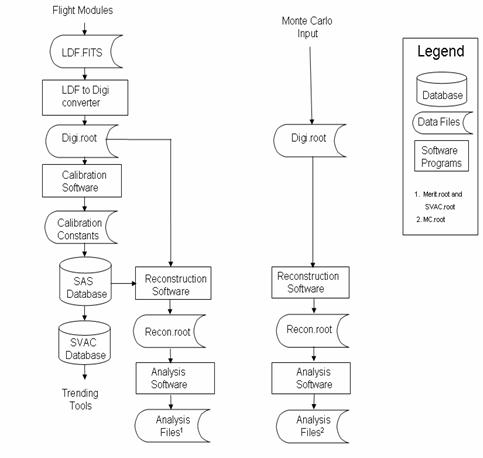
Figure
22: Data
Analysis Process Flow
TKR
reconstruction is an iterative process using information from both the CAL and
TKR. The TKR reconstruction method adopts the following four-step procedure
(please see Figure 23 and Figure 24)
1. Form
“Cluster Hits”
Done by converting the hit strips to
positions. Adjacent hit strips are merged to form a single hit.
2. Pattern
Recognize individual tracks
Done by associating cluster hits
into candidate tracks. Individual track energies are assigned to aid in track recognition.
3. “Fit”
Track to obtain track parameters
Inherently two-dimensional cluster
locations are processed to determine three-dimensional position and direction. The errors are
estimated then the energy calculations are used to help with track fitting.
4. “Vertex”
fit tracks
The common intersection point of fit
tracks is determined, and a position and direction is calculated.
For cosmic rays, the first hit plane determines the “vertex” location. The diagrams
presented in Figure
24 illustrate how a cosmic ray event can have more than one track and even
multiple vertices.

Figure
23: Four TKR
Reconstruction Steps (Block Diagram)

Figure
24:
Four Steps of TKR
Reconstruction (Illustrated)
Iterative
Recon allows parts of the TKR Reconstruction software to be called more than
once per event. The overview is shown in Figure 25. In particular, existing pattern
recognition tracks can be refit and the vertex algorithm re-run.
The
Iterative Recon provides the CAL Recon with sufficient tracking information to
get an improved energy estimate, which can be fed back to the track fit and
vertexing algorithms. The process can be repeated as many times as the user
likes (in principle) but the default is two passes.
Figure
25: Iterative
TKR Reconstruction Algorithms (Block Diagram)
The
clustering algorithms group strips with adjacent hits to form a cluster. TkrClusterAlg
takes the strip hits to calculate the center position to use in track fitting.
The digi.root file (please refer to Digi.root in section 7.2.2) provides clustering of the hit strip numbers, and
Time over Threshold (ToT).
The
clustering algorithms apply the TKR calibration data to account for
hot/dead/sick strips and merges clusters with known dead strips between them.
It also decides whether to add known hot strips to clusters.
The
result of TkrClusterAlg is a list of clusters in TDS with associated XYZ
coordinates and the value of ToT associated with these strips. This information
is used in the next step by TkrFindAlg.
The
output of track finding is an ordered list of candidate tracks to be fit. TkrPatCand,
contained in a TkrPatCandCol Gaudi object vector, outputs:
·
Estimated track parameters for the candidate
track (position, direction);
·
The energy assigned to the track;
·
Track candidate “quality” estimates, and;
·
Starting tower / plane information.
TkrPatCand contains the Gaudi object vector
of TkrPatCandHits for each hit
(cluster) associated with the candidate track. Any cluster associated with this
hit is needed for the fit stage.
All
are stored in the TDS.
TkrFindAlg
associates clusters into candidate tracks. Three approaches exist within the TkrRecon
package, as described in Table 17.
Table
17: TKR
Reconstruction Clustering Methods
|
|
|
|
|
|
Combo
|
Track
by track. Combinatoric search through space points to find candidates.
|
Simple
to understand (although details add complications)
|
Finding
“wrong” tracks early in the process throws off the rest of the track finding
by mis-associating hits. Can be quite time consuming depending upon the depth
of the search.
|
|
Link
and Tree
|
Global
pattern recognition. Associate hits into a tree like structure.
|
Optimized
to find tracks in entire event, less susceptible to miss associating hits.
|
Can
be quite time consuming.
|
|
Neural
Net
|
Global
pattern recognition. Links nearby space points forming “neurons.”
|
Optimized
to find tracks in entire event, less susceptible to miss associating hits.
|
Can
be quite time consuming. Operates in 2D and then requires mating to get 3D
track.
|
Also:
“Monte Carlo” pattern recognition exists for testing, fitting and vertexing.
There
are two basic Combinatoric strategies for track finding: CAL based or Blind
search. CAL based is used when there is enough CAL energy present to use the energy
centroid. When there is too little CAL energy we use only Track Hits, and make
a “Blind” search.
Table 18 differentiates between the types of
combinatoric track finding methods available to ComboFindTrackTool. In either case its starting plane is
always the one furthest from the CAL. It works to combine clusters in adjacent
X-Y planes to form 3D space points.
Table
18: TKR
Reconstruction Combinatoric Track Finding Methods
|
|
|
|
|
CAL
Energy Present
|
Sufficient
CAL energy, about 42 MeV.
|
Track
fit uses the CAL centroid by first attempting to connect the hit with CAL centroid.
It connects the first two hits, then projects and adds hits along the track
within the search region. The search region is set by propagating the track
errors through the GLAST geometry. Please see Figure
26.
|
|
Blind
search
|
Insufficient
CAL energy.
|
The
first hit found is tried in combinatoric order. The 2nd hit is selected in
combinatoric order. The first two hits are used to project into next plane,
and a 3rd Hit is searched for. If a 3rd hit is found the track is built by
“finding – following.”
|
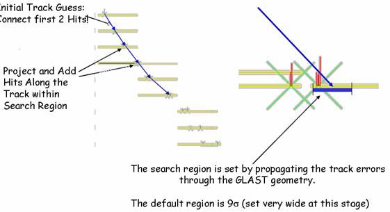
Figure
26:
Combinatoric Pattern Recognition: ComboFindTrack Tool
The
next step is for the TkrReconAlg to fit the candidate tracks using the
parameters of X, Y and the slopes of X and Y. It tracks the parameter error
matrix (parameter errors and correlations) and measures of the quality of the
track fit using the Kalman filter method.
The
filter process starts at the conversion point, but we want the best estimate of
the track parameters at the conversion point. This requires propagating the
influence of all the subsequent hits backwards to the beginning of the track,
essentially running the filter in reverse. This is called the smoother, and the
linear algebra is similar:
Residuals: r(k) = X(k) -Pm(k)
Covariance of r(k): Cr(k) = V(k)
-C(k)
Then: X2 =
r(k)TCr(k)-1r(k)
for the kth step
A
pair conversion results in 2 primary tracks,
but one track could be lost due to:
·
Low energy (track must cross three planes);
·
Tracks from pair conversion don’t separate for
several planes; and,
·
Track separation due to multiple scattering.
In
addition, wrong vertex associations could occur because secondary tracks may be
associated with primary tracks but are not part of the g conversion process.
The
vertexing algorithm attempts to associate “best” track (from track finding)
with one of the other found tracks by finding “the” vertex and returning
unassociated (“isolated”) tracks as single prong vertices. It determines the
reconstructed position of the conversion and the reconstructed direction of the
conversion. Currently two methods available, as listed in Table 19.
In
the presence of charged particles only, the vertex is considered to be at the
first plane hit.
Table
19: TKR
Reconstruction Vertexing Tools
|
|
|
|
|
“Combo”
(default)
|
Uses
track Distance of Closest Approach (DOCA) to associate tracks.
|
1.
The vertex is determined at two tracks’ Distance of Closest Approach (DOCA).
2.
The first track is the “best” track from track finding/fitting algorithms.
3.
It is looped through “other” tracks looking for best match:
·
Smallest DOCA
·
Weighting factors:
·
Separation between the starting points of the
two tracks
·
Track energy
·
Track quality
4.
It calculates vertex quantities:
·
Vertex Position: Midpoint of DOCA vector
·
Vertex Direction: Weighted vector sum of
individual track directions
Not
a true HEP Vertex Fit
|
|
Kalman Filter
|
Kalman Filter
|
|
The
output from the vertexing algorithms is an ordered list of vertices with the
following TkrVertex objects
contained in a Gaudi Object Vector:
·
The vertex track parameters (x, mx,
y, my);
·
The vertex track parameter covariance matrix;
·
The vertex energy;
·
The vertex quality;
·
The first tower/plane information; and,
·
Gaudi reference vector to the tracks in the
vertex.
The
first vertex in the list is the “best” vertex, and the rest are mostly associated
with an “isolated” track.
By default, the track finding and fitting
assume that all tracks are electrons. This has two consequences: It will use
the electron hypothesis to calculate the energy loss in the tracker, and it can
use the total energy deposited in the calorimeter as a reliable estimate of the
true track energy.
However,
for most of the Integration and Test period we will have surface muons in the
detector. Using the electron hypothesis to find and fit muon tracks has two
consequences: The energy loss in the tracker will be vastly overestimated as a
muon loses much less energy than an electron per radiation length, and the
energy deposited in the calorimeter is no longer a good estimate of the true
track energy. A MIP leaves about 90 MeV in the calorimeter.
This
means that a 5 GeV muon, for example, will be treated as a 90 MeV electron in the
track finding and fitting. Note that this will affect the track reconstruction
strategy. For a 90 MeV electron only the first few points on the track are used
to estimate the incident direction, the assumption being that multiple
scattering will make the points further down on the track useless.
The
track reconstruction has the ability to use a muon hypothesis. This means the
energy loss will be calculated correctly. However, because the energy deposited
in the calorimeter can no longer be used as an estimator for the true track
energy, we need to set a fixed minimum track energy. The maximum of the minimum
track energy and the energy deposited in the calorimeter will then be used.
Studies are underway to find the precise minimum track energy to use.
Preliminary studies indicate that it will be in the range of 500 MeV to a few
GeV.
For
all runs with surface muons during Integration and Test we will use the muon
hypothesis for the track finding and fitting.
Another
point to note is that for a specific event only one particle hypothesis can be
used. This means that for runs with photons, like VDG runs, where we will
specify the electron hypothesis and set the minimum track energy to 4 MeV, any
surface muon passing through the detector at the same time will also be
reconstructed as an electron with a track energy which is the greater of either
4 MeV or the energy deposited in the calorimeter. One should keep this in mind
when comparing MIP distributions from VDG runs and normal surface muon runs.
MC
simulations are run for both simulated cosmic rays at sea level and photons
generated by a Van De Graaff generator.
MC
simulations on thresholds and noise are taken for data analysis purposes, and
are also described here.
Simulated
g photons are derived from real proton / Lithium 7
collisions according to Figure 27.

Figure
27: Simulation
of VDG Gammas – Simulated Particle Source Generation
For
MC simulation, there is no Li target – only the g are simulated, with an energy spectrum having the main
distribution at 14.6 MeV and a 17.6 MeV line spectrum. The ratio of numbers of
events at 17.6 MeV / number of events at 14.6 MeV is 2:1.
The
shielding is defined as a simulated iron cylinder with radius of 26 mm and
thickness of 1.25 mm (7% X0). The X position = -200
mm; the Y position = 200 mm; the Z position = 636 mm, ~ 3mm above the TKR. The
energy spectrum is angular-dependent.
Note
that g photons which convert in
the Fe shield generate an unwanted experimental background of charged
particles.
The
default scenario program name is surface_muons (muons at the earth’s surface).
It models energy / angle correlations and has a spectrum to include events
below 1 GeV. It can produce a small number of unphysical, low energy events
that are platform dependent. There
is no simulation of particle showers.
Figure 28 shows the distribution of kinetic
energy vs. particle flux for surface_muons.
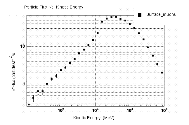
Figure
28: Particle
Flux vs. Kinetic Energy for surface_muon Source
The TKR
occupancy in MC is usually set at 5 x 10 -5 /
strip, meaning that one should expect about 3 noisy hits per tower, on average
(5 x 10 -5
/strip x 1536 strips x 36 planes per tower).
This section is intended to guide users in
the usage of the existing data analysis variables. It is impossible to provide
a recipe for data analysis, but the idea is to illustrate how to use the
information in the data analysis files.
A MIP selection can involve information from
TKR, CAL and ACD.
The most naïve search is for a single
straight track, with one hit in each TKR plane, that when extrapolated to the CAL,
deposits about 11 MeV in each crystal layer.
The SVAC file has hits per plane and clusters
per plane for each tower while the Merit ntuple has clusters associated to
tracks for all towers.
Care needs to be exercised when using variables
such as TkrTrackLength. This variable measures an extrapolated length
from the first hit plane to the grid by dividing Tkr1Z0 (Z position at
first hit of track1) by Tkr1ZDir (direction cosine for track1). Thus,
for a situation illustrated in Figure 29, both track lengths are equal.
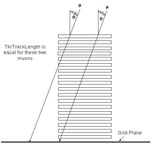
Figure 29: TrkTrackLength Example of Easily Misinterpreted Data
Note
that when extrapolating a track into the CAL, sometimes the track will traverse
different amounts of material even if it is a straight track. The reason is
depicted in Figure 30. In this case there is an offset
between successive CAL layers, so an on-axis muon, contrary to naive intuition,
may hit every other plane.
Figure
30: A Charged
Particle’s Path is Parallel to the Z Axis and only Strikes Every Other Crystal
Note
that when we have even and odd bays populated with towers, it is important to
verify timing settings because cable lengths will be different.
Please see the following references for
additional information.
Appendix A
- eLog
The eLog makes available all the run data information for
any of the electronics tests run on the LAT components.
There are two eLog displays with similar names described
here: The GLAST Shift Index and the Run Selection Index.
A.1.
Shift
Logbook Index
The Shift Log Index’s calendar, shown below in Figure 31, accesses day-to-day activities at SLAC.
Its URL is: http://www.slac.stanford.edu/cgi-wrap/eLog.pl/index
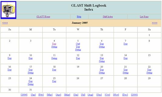
Figure 31: GLAST Shift Log Index
This access route to the data displays all the same
information categories as the query form, but the only sort function is time of
test, e.g., the day shift on Wednesday, 01/05/05. The categories are described
below. Selecting List Runs from the Index page displays the GLAST Shift Logbook Shift
Run Info menu, shown below in Figure 32.
A.2.
Run
Selection Index
The Run Selection Index is used to retrieve run data by
specifying specifics you enter, such as the particle type and / or the site
where the test was run and / or instrument type (the unit under test) serial
number, and / or date of test, etc., and is shown in Figure 32.
Its URL is: http://www.slac.stanford.edu/cgi-wrap/eLog.pl/list
·
Asterisk (*)
wildcards are allowed for queries.
·
Fields
are not case sensitive.
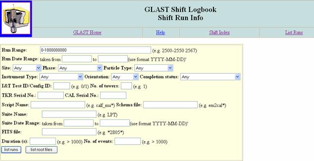
Figure 32: Logbook
Shift Run Info
The fields from Figure 32: Logbook Shift Run
Info are described below in Table 20. The table is divided into two parts:
the top half lists fields most used for data analysis; the bottom half is for
subsystem experts.
Table 20: Logbook
Shift Run Menu Fields
|
|
|
|
|
Most-used
fields for data analysis.
|
|
Run Range
|
Numeric * wildcard allowed
|
A range or set of run numbers
|
|
Run Date Range
|
YYYY-MM-DD * wildcard allowed
|
A range or set of runs by date
|
|
Particle type
|

|
Photon = Van de
Graaff g; peaks at 14.6 MeV and 17.6
MeV with a ratio of 2:1.
Cosmics = cosmic rays
Charge injection is for subsystem experts
|
|
|
|
|
|
Orientation
|

|
Orientation of instrument (important for cosmic ray
runs). Photon tests are always horizontal.
|
|
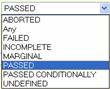
Completion status
|
|
Test status. Indicates that a test executed
successfully or unsuccessfully – not an indicator of the equipment’s status.
|
|
No. of Towers e.g.1
|
1 - 16
|
Number of towers in the grid.
|
|
TKR Serial No.
|
Normal TKR range is: TKR FMA to TKR FM16
|
TKR unit. Same as instrument type.
|
|
CAL Serial No.
|
Normal CAL range is: FM101 to FM118
|
CAL unit. Same as instrument type.
|
|
Duration(s)
|
Numeric value in seconds. < > allowed, e.g., < 1000 or >1000
|
Test duration in seconds.
|
|
No. of events
|
Numeric value. < > allowed, e.g., < 1000 or
>1000
|
Number of events in the runs.
|
|
I&T Test ID/Config ID (e.g. 0/1)
|
|
End-to-end test IDs
|
|
Fields for
subsystem experts.
|
|
Site
|

|
Test site where data was collected.
|
|
Phase
|
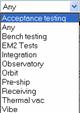
|
Test phase during LAT integration.
|
|
Instrument type
|
|
Flight hardware CAL range is: FM 101, FM 102 …FM 118
Flight
hardware TKR range is: TKR FMA to TKR FM16
Superseded- please do not rely on this.
Use Serial Numbers.
|
|
Script name (e.g. calf_mu*):
|
|
Test script
|
|
Schema File (e.g. em2cal*):
|
|
Description of register configurations
|
|
Suite name (e.g. LPT):
|
|
A group of tests bound together
|
|
Suite Date Range
|
YYYY-MM-DD
|
Specify a range of test suites.
|
|
FITS file
|
Numeric value that corresponds to run numbers.
Wildcards allowed.
|
Raw data
|
Table 21: Logbook Shift Run Menu Active Buttons
|
|
|
|
|

|
Get runs according to menu choices.
|
View shown in Figure
33
|
|

|
ftp path for
test-run created root files at SLAC for analysis.
|
Will be updated to show URLs for the test-run created
root files.
|
A.3.
List Runs
Selecting List Runs
from either the Shift Log Index or from the Run Selection Index displays the
table of information shown in Figure 33.
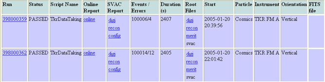
Figure 33:
List Runs Table
The fields in Figure 33: List Runs Table are described in Table 22.
Table 22: List Runs Fields
|
|
|
|
Run
|
Summary run information. All information fields from
Run Info (Table
20) plus
processing files package.
|
|
Status
|
Flag for test results
|
|
Script Name
|
Name of LATTE script used for the run
|
|
Online Products
|
Links to all files created by LATTE for the test run.
|
|
SVAC Report
|
Links to: http, .ps or .pdf
versions of digi, recon and config file data quality reports.
Digi: digi file details, run results, test settings.
Recon: details of recon software and result displays.
Config: Details of CAL, TKR and ACD configuration settings while
under test.
Digi and Recon reports are used in offline data
analyses to identify apparent problems in cosmic ray muon and VDG data.
|
|
Events/Errors
|
Number of events in the test / number of errors in the
test
|
|
Duration (s)
|
Number of seconds the test lasted.
|
|
Root files
|
Links to: digi, recon, merit, SVAC data analysis
files.
Requires Root to visualize data. Please see the
Instrument Analysis main page at: http://www-glast.slac.stanford.edu/IntegrationTest/SVAC/Instrument_Analysis/Instrument_Analysis.html
|
|
Start
|
Date and time test started
|
|
Particle type
|
Particle type of test run (cosmics, photons)
|
|
Orientation
|
Unit orientation (vertical or horizontal)
|